Infer.NET user guide : Learners : Bayes Point Machine classifiers
The Bayes Point Machine: A probabilistic model for classification
We are interested in finding a general and robust procedure to predict the class  to which an instance of interest belongs, given relevant feature values
  of this instance and the information in
  , the training set of observed class labels and corresponding feature values.
It can be shown that the only coherent solution to the classification problem is to provide the predictive distribution  over classes, conditional on and
  . In the following we provide a direct specification of the predictive distribution
  based on a set of assumptions. The derived classification model thus falls into the discriminative paradigm.
Binary classification
For simplicity, we will start by describing the model for the case of two class labels  . The model is defined by the following assumptions:
Assumption 1: The feature values are always fully observed.
This means that it must always be possible to compute all feature values. If features are missing for some instances, you will either have to fill in the missing values in a pre-processing step, or use a different model for classification.
Assumption 2: The order of instances does not matter.
That is, instances are assumed to be exchangeable. As a result of this assumption, the predictive distribution  is characterized, for any given , by the same latent parameters
  , also referred to as weights.
If the predictive distribution varies with time, for example in the stock market, then you will need to expand to include time information or use a different model for classification (such as a time-series model).
Assumption 3: The predictive distribution is a linear discriminant function.
We assume the predictive distribution to have a parametric density of the form

where  is called the score of the instance.
Assumption 4: Additive Gaussian noise.
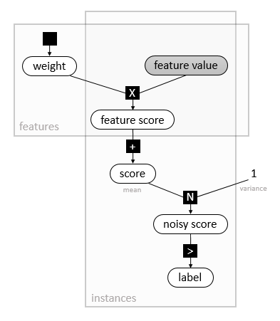
To allow for measurement and labelling error, we add Gaussian noise to the score:
 with
with  and
and 
This is also known as a probit regression model.
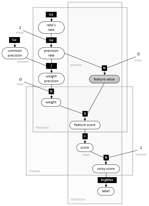
The model up to this point, represented as a factor graph, is depicted below:
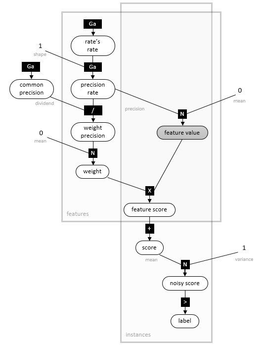
Assumption 5: Factorized heavy-tailed prior distributions over weights .
Finally, by specifying the prior distribution  , we complete the probabilistic model for the Bayes Point Machine classifier. We use a heavy-tailed prior, a normal distribution whose precision is itself a mixture of Gamma-Gamma distributions (as illustrated in the factor graph below, where
  denotes a Gamma density for given shape and rate). Compared with a Gaussian prior, the heavy-tailed prior is more robust towards outliers, i.e. feature values which are far from the mean of the weight distribution, 0. It is invariant to rescaling the feature values, but not invariant to their shifting (to achieve the latter, the user must add a bias - a constant feature value - for all instances). Due to the factorized structure of , features should be as uncorrelated as possible.
Multi-class classification
The multi-class model is very similar to the described binary Bayes Point Machine model. Instead of a single linear discriminant function, there are now  functions with their respective weight vectors
  and scores
  , one for each class
  . The maximum (noisy) score then determines the class .
Assumption 6: Class labels have no inherent ordering.
The multi-class model assumes that the class labels have no inherent ordering, and is thus invariant to permuting the set of labels. If the labels in your problem have an order, then you can still use this model, even though you might benefit from a different model.
With appropriate symmetry-breaking, using the multi-class model with 2 classes is equivalent to the binary model described above. However, an exception will be thrown if you try this. Finally, the computational cost of prediction in the multi-class model is quadratic in the number of classes , making it less ideal a choice where is large.
Source code
The Infer.NET code for the previously described classification models lives in the Learners/ClassifierModels project. The project uses the Infer.NET compiler to generate dedicated training and prediction algorithms from the models.
References
- Herbrich, R., Graepel, T. and Campbell, C. (2001). Bayes Point Machines. Journal of Machine Learning Research 1, 245-279.
- Minka, T. (2001). Expectation Propagation for approximate Bayesian inference. Uncertainty in Artificial Intelligence, 2001, 362-369.